All Basic Excel Formula (एक्सेल के सभी सूत्रों को समझे और जाने )
Basic Excel Formulas
- English Hindi(हिंदी में )
- Sum जोड़ करे
- If and Nested if कंडीशन (शर्त)
- Percentage प्रतिशत केसे निकाले
- Subtraction घटाना सीखे
- Multiplication गुणा करना सीखे
- Date (तारीख जाने /तारीख जोड़ना या घटना सीखे ,साल निकलना सीखे )
- Array
- Count (गणना करे )
- Average (औसत निकाले )
- Sumif (शर्तो के साथ जोड़ना सीखे )
- Trim नाम श्रृंखला को काटना/छांटना सीखे )
- Left बाएँ से नाम श्रृंखला को निकाले
- Mid मध्य से
- Right दायें से नाम श्रृंखला को निकाले
- Vlookup वर्टीकलि सारणी को ढूढ कर चयनात्मक ऑब्जेक्ट विशेष का पता करना
- Randomize अनियमित तरीके से डाटा का पता करे
- Learn Excel more effectively , I have written a list of essential formulas, keyboard shortcuts, and other small tricks and functions you should know.
Sum Function Shortcut for Sum (Alt+=)
All Excel formulas starts with the equals sign, =,
The SUM formula in Excel is basic formulas that you can enter into a spreadsheet, allowing you to find the sum (or total) of two or more values. To perform the SUM formula, enter the values you'd like to add together using the format, =SUM(value 1, value 2, etc).
The value you enter in Sum formula it may by number value or may be cell reference
- Example: to find the SUM of 50 and 75, for example, type the following formula into a cell of your spreadsheet: =SUM(50,75). Press "Enter," and the cell will produce the total of both numbers: 125.
- To find the SUM of the values in cells B6 and B9, for example, type the following formula into a cell of your spreadsheet: =SUM(B6, B9). Press "Enter," and the cell will produce the total of the numbers currently filled in cells B6 and B9. result value shown in cell B10
-

Also you can press short cut key for sum formula for this select your last cell B10 then press and hold Alt key and type +/= key you will get your sum formula there.
If condition
The IF formula in Excel is denoted =IF(logical_test, value_if_true, value_if_false). This allows you to enter a text value into the cell "if" something else in your spreadsheet is true or false. For example,
Here Field name "Employee With Total Sale" belong to F14 cell
Result of True:Here by if condition we are checking total sale of f14 amount is grater then 300000 or not if it true then the value result of True will shown which are written "Very Good". other wise .jums to false value result
Result of False:Here by if condition we are checking total sale of f14 amount is not grater then 300000 then result of false will shown which are written "Not Good".
that are mention in Sale Performance Field.

. The formula: IF(logical_test, value_if_true, value_if_false
Note: Make sure your Logical_Test value is in quotation marks,if it is in text form and both value should be separated with the "," Comma Symbol as highlighted in above formula

Percentage % Formula
To perform the percentage formula in Excel, enter the cells you're finding a percentage for in the format,
Formula of Percentage = value1/Value2*100
Example Ram Achieved 590 Marks out of 600 then, to find oput percentage there are two method to get percentage
One, is given this formula first write =590/600*100 then press "Enter"

Second, is by using % function of excel, before using this type divide value
=590/600 then if you enter then it shows result in decimal number value to converting in percentage % form click on % symbol.
Go to Home tab- Number tools Group to convert the resulting decimal value into to a percentage form


Excel makes it easy to convert the value of any cell into a percentage so need to worry about this.
For regular use of this do your basic setting to convert a cell's value into a percentage is that mention under Excel's Home tab. Select this tab, highlight the cells where you would like to convert to a percentage,
Keep in mind if you're using other formulas, such as the division formula (denoted =A1/B1), to return new values, your values might show up as decimals by default. Simply highlight your cells before or after you perform this formula, and set these cells' format to "Percentage" from the Home tab -- as shown above.
Subtraction Formula(=Sum(Value1,-Value2)
How to perform the subtraction formula in excel,its very simple as generally by doing "-" Minus symbol.
Note: In Excel there is any (Subtraction or Minus) function not available in excel
so there are two methods to do subtraction in excel
One method simply we have to do manually by =A-B,
=(First higher value - Second Lower Value) .
Example Cell E34-F34
E34 belong to Total Majdoori F34 cell belong to Expenses of tea at work place so the net income of labour are 15000-150=14850


Second method is by keeping negative symbol in sum formula
the format is , =SUM(A1, - B1).
Suppose in cell A1 we have 100 and in B1 we have 90 then what are the difference of both so will use second method =sum(A1,-B1) result will be 10
Labour example with table

Multiplication(*)
It is also as like subtraction for there is any specific formula with name multiply instead of that here one for function is available in excel that does the work of multiplication .that are our our second method,
Here see the first method.
=Value1*value2 ,
here value1 in below table is in Per day Payment field 500 and value 2 is in number of days field that is 30 to total majdoori =500*30 which are in cell value c34*d34 then press "Enter"

Second Method ,Excel providing us facility of multiplication by using Product formula ,here in excel instead of Multiplication we will use PRODUCT formula
let see

=PRODUCT(VALUE1,VALUE2) ,Here you did not need to apply Asterisk(*) symbol for multiplication ,this function automatically do this work.
here in above table you see B11 and C11 are multiplying by PRODUCT function and will return result of multiplication.
Division(/)
How to perform the division formula in Excel, enter the cells you're dividing in the format, =D11/E11. This formula uses a forward slash, "/," to divide cell D11 by cell E11.
For example, here D11 belong to Monthly Labour Payment field and E11 belong to Working Day field find out how much Per day labour cost is. so we use Dividation formulation by using this method

Press Enter, and your desired result should appear in the cell you initially highlighted.
DATE
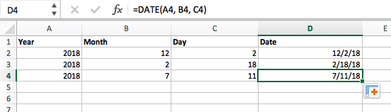
The Excel DATE formula is denoted =DATE(year, month, day). This formula will return a date that corresponds to the values entered in the parentheses -- even values referred from other cells. For example, if A1 was 2018, B1 was 7, and C1 was 11, =DATE(A1,B1,C1) would return 7/11/2018.
Creating dates in the cells of an Excel spreadsheet can be a fickle task every now and then. Luckily, there's a handy formula to make formatting your dates easy. There are two ways to use this formula:
- Create dates from a series of cell values. To do this, highlight an empty cell, enter "=DATE," and in parentheses, enter the cells whose values create your desired date -- starting with the year, then the month number, then the day. The final format should look like this: =DATE(year, month, day). See how this looks in the screenshot below.
- Automatically set today's date. To do this, highlight an empty cell and enter the following string of text: =DATE(YEAR(TODAY()), MONTH(TODAY()), DAY(TODAY())). Pressing enter will return the current date you're working in your Excel spreadsheet.
In either usage of Excel's date formula, your returned date should be in the form of "mm/dd/yy" -- unless your Excel program is formatted differently.
Array
An array formula in Excel surrounds a simple formula in brace characters using the format, {=(Start Value 1:End Value 1)*(Start Value 2:End Value 2)}. By pressing ctrl+shift+center, this will calculate and return value from multiple ranges, rather than just individual cells added to or multiplied by one another.
Calculating the sum, product, or quotient of individual cells is easy -- just use the =SUM formula and enter the cells, values, or range of cells you want to perform that arithmetic on. But what about multiple ranges? How do you find the combined value of a large group of cells?
Numerical arrays are a useful way to perform more than one formula at the same time in a single cell so you can see one final sum, difference, product, or quotient. If you're looking to find total sales revenue from several sold units, for example, the array formula in Excel is perfect for you. Here's how you'd do it:
- To start using the array formula, type "=SUM," and in parentheses, enter the first of two (or three, or four) ranges of cells you'd like to multiply together. Here's what your progress might look like: =SUM(C2:C5
- Next, add an asterisk after the last cell of the first range you included in your formula. This stands for multiplication. Following this asterisk, enter your second range of cells. You'll be multiplying this second range of cells by the first. Your progress in this formula should now look like this: =SUM(C2:C5*D2:D5)
- Ready to press Enter? Not so fast ... Because this formula is so complicated, Excel reserves a different keyboard command for arrays. Once you've closed the parentheses on your array formula, press Ctrl+Shift+Enter. This will recognize your formula as an array, wrapping your formula in brace characters and successfully returning your product of both ranges combined.
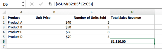
In revenue calculations, this can cut down on your time and effort significantly. See the final formula in the screenshot above.
Same can also Apply by using SUMPRODUCT formula
COUNT
How to perform the COUNT function in excel,the COUNT formula in Excel is denoted =COUNT(Start Cell:End Cell). This formula will return a value that is equal to the number of entries found within your desired range of cells. For example, if there are eight cells with entered values between A1 and A10, =COUNT(A1:A10) will return a value of 8.
The COUNT formula in Excel is particularly useful for large spreadsheets, wherein you want to see how many cells contain actual entries. Don't be fooled: This formula won't do any math on the values of the cells themselves. This formula is simply to find out how many cells in a selected range are occupied with something.
By using this table we will understand Count function to count number of students

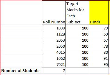
Count function always counts the number available in cell range it may be in text form or in number form
Note : this function does not add the the data or value
AVERAGE
How to perform the average formula in Excel, enter the values, cells, or range of cells of which you're calculating the average in the format, =AVERAGE(number1, number2, etc.) or =AVERAGE(Start Value:End Value). This will calculate the average of all the values or range of cells included in the parentheses.
Finding the average of a range of cells in Excel keeps you from having to find individual sums and then performing a separate division equation on your total. Using =AVERAGE as your initial text entry, you can let Excel do all the work for you.
For reference, the average of a group of numbers is equal to the sum of those numbers, divided by the number of items in that group.
SUMIF
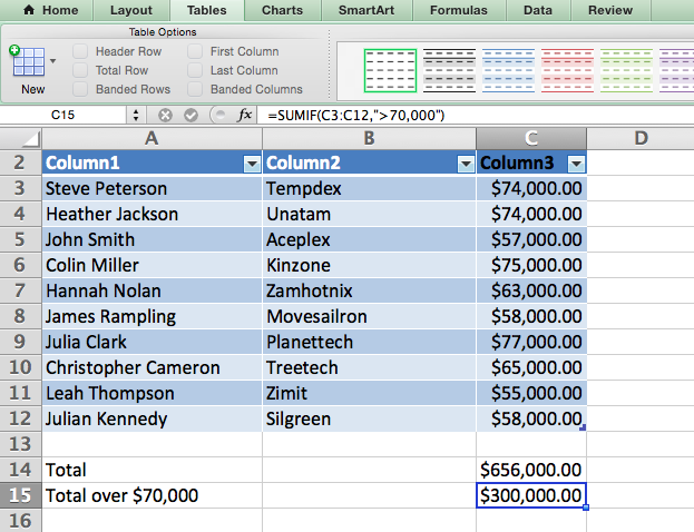
How to Perform the SUMIF Formula in Excel,The SUMIF formula in Excel is denoted =SUMIF(range, criteria, [sum range]). This will return the sum of the values within a desired range of cells that all meet one criterion. For example, =SUMIF(C3:C12,">70,000") would return the sum of values between cells C3 and C12 from only the cells that are greater than 70,000.
Let's say you want to determine the profit you generated from a list of leads who are associated with specific area codes, or calculate the sum of certain employees' salaries -- but only if they fall above a particular amount. Doing that manually sounds a bit time-consuming, to say the least.
With the SUMIF function, it doesn't have to be -- you can easily add up the sum of cells that meet certain criteria, like in the salary example above.
- The formula: =SUMIF(range, criteria, [sum_range])
- Range: The range that is being tested using your criteria.
- Criteria: The criteria that determine which cells in Criteria_range1 will be added together
- [Sum_range]: An optional range of cells you're going to add up in addition to the first Range entered. This field may be omitted.
In the example below, we wanted to calculate the sum of the salaries that were greater than $70,000. The SUMIF function added up the dollar amounts that exceeded that number in the cells C3 through C12, with the formula =SUMIF(C3:C12,">70,000").
TRIM
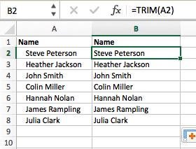
The TRIM formula in Excel is denoted =TRIM(text). This formula will remove any spaces entered before and after the text entered in the cell. For example, if A2 includes the name " Steve Peterson" with unwanted spaces before the first name, =TRIM(A2) would return "Steve Peterson" with no spaces in a new cell.
Email and file sharing are wonderful tools in today's workplace. That is, until one of your colleagues sends you a worksheet with some really funky spacing. Not only can those rogue spaces make it difficult to search for data, but they also affect the results when you try to add up columns of numbers.
Rather than painstakingly removing and adding spaces as needed, you can clean up any irregular spacing using the TRIM function, which is used to remove extra spaces from data (except for single spaces between words).
- The formula: =TRIM(text).
- Text: The text or cell from which you want to remove spaces.
Here's an example of how we used the TRIM function to remove extra spaces before a list of names. To do so, we entered =TRIM("A2") into the Formula Bar, and replicated this for each name below it in a new column next to the column with unwanted spaces.
Below are some other Excel formulas you might find useful as your data management needs grow.
LEFT, MID, and RIGHT
Let's say you have a line of text within a cell that you want to break down into a few different segments. Rather than manually retyping each piece of the code into its respective column, users can leverage a series of string functions to deconstruct the sequence as needed: LEFT, MID, or RIGHT.
LEFT
- Purpose: Used to extract the first X numbers or characters in a cell.
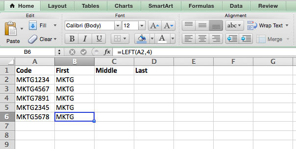
- The formula: = LEFT(text, number_of_characters)
- Text: The string that you wish to extract from.
- Number_of_characters: The number of characters that you wish to extract starting from the left-most character.
In the example below, we entered =LEFT(A2,4) into cell B2, and copied it into B3:B6. That allowed us to extract the first 4 characters of the code.
MID
- Purpose: Used to extract characters or numbers in the middle based on position.
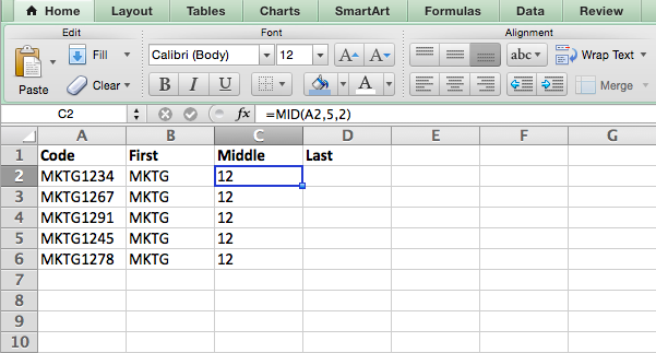
- The formula: =MID(text, start_position, number_of_characters)
- Text: The string that you wish to extract from.
- Start_position: The position in the string that you want to begin extracting from. For example, the first position in the string is 1.
- Number_of_characters: The number of characters that you wish to extract.
In this example, we entered =MID(A2,5,2) into cell B2, and copied it into B3:B6. That allowed us to extract the two numbers starting in the fifth position of the code.
RIGHT
- Purpose: Used to extract the last X numbers or characters in a cell.
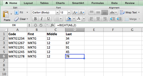
- The formula: =RIGHT(text, number_of_characters)
- Text: The string that you wish to extract from.
- Number_of_characters: The number of characters that you want to extract starting from the right-most character.
For the sake of this example, we entered =RIGHT(A2,2) into cell B2, and copied it into B3:B6. That allowed us to extract the last two numbers of the code.
VLOOKUP
This is very useful function,it's especially helpful when you have two sets of data on two different spreadsheets, and want to combine them into a single spreadsheet.
Note: When using this formula, you must be certain that at least one column must be unique and available in both spreadsheets.
- The formula: VLOOKUP(lookup value, table array, column number, [range lookup])
- Lookup Value: The identical value you have in both spreadsheets. Choose the first value in your first spreadsheet. In Sprung's example that follows, this means the first email address on the list, or cell 2 (C2).
- Table Array: The range of columns on Sheet 2 you're going to pull your data from, including the column of data identical to your lookup value (in our example, email addresses) in Sheet 1 as well as the column of data you're trying to copy to Sheet 1. In our example, this is "Sheet2!A:B." "A" means Column A in Sheet 2, which is the column in Sheet 2 where the data identical to our lookup value (email) in Sheet 1 is listed. The "B" means Column B, which contains the information that's only available in Sheet 2 that you want to translate to Sheet 1.
- Column Number: The table array tells Excel where (which column) the new data you want to copy to Sheet 1 is located. In our example, this would be the "House" column, the second one in our table array, making it column number 2.
- Range Lookup: Use FALSE to ensure you pull in only exact value matches.
- The formula with variables from Sprung's example below:
- =VLOOKUP(A22,Row Data of Student!$i$2:$y$17,11,0)


In this example, Sheet 1 and Sheet 2 contain lists describing different information about the same people, and the common thread between the two is their email addresses. Let's say we want to combine both datasets so that all the house information from Sheet 2 translates over to Sheet 1. Here's how that would work:
RANDOMIZE
What are the use of Randomize function in excel, RANDOMIZE formula to shuffling a piece of cards.
In marketing, you might use this feature when you want to assign a random number to a list of contacts -- like if you wanted to experiment with a new email campaign and had to use blind criteria to select who would receive it. By assigning numbers to said contacts, you could apply the rule, “Any contact with a figure of 10 or above will be added to the new campaign.”
- The formula: RAND()
- Start with a single column of contacts. Then, in the column adjacent to it, type “RAND()” -- without the quotation marks -- starting with the top contact’s row.
- For the example below: RANDBETWEEN(bottom,top)
- RANDBETWEEN allows you to dictate the range of numbers that you want to be assigned. In the case of this example, I wanted to use one through 10.
- bottom: The lowest number in the range.
- top: The highest number in the range,
- Formula in below example: =RANDBETWEEN(1,10)

Comments